Quantum 1/f Proximity Effect in Nanotechnology
by
Peter H. Handel*
Department of Physics and Astronomy, Univ. of Missouri-St. Louis, St. Louis MO 63121
*[email protected]
http://www.umsl.edu/~handel
This is a draft paper for the
Eighth
Foresight Conference on Molecular Nanotechnology.
The final version has been submitted
for publication in the special Conference issue of Nanotechnology.
Abstract
This paper shows that in certain conditions fundamental 1/f noise in a semiconductor sample is increased by the presence of another similar current-carrying sample located in the close vicinity. This proximity effect is described by simple formulas derived here. The paper explains the connection between the coherent and conventional quantum 1/f effect. On this basis the proximity effect is introduced for the first time. It is shown to be important in the transition region between coherent and conventional quantum 1/f effect. This is just the region corresponding to nano-scale structures and devices. Therefore, the effect will be important in nanotechnology.
I. Introduction
Electrical currents in nanostructures of any nature exhibit unusual 1/f noise. They are in the transition region between two different components of the fundamental quantum 1/f noise. This transition region between the coherent and conventional quantum 1/f effects is described by the relation
| aH = aconv/(1+s) + acohers/(1+s) = (4a/3p)(Dv/c)2/(1+s) + (2a/p)s/(1+s) |
(1) |
for the quantum 1/f parameter aH, where s is a parameter that governs the transition. The parameter s depends on the concentration n of carriers and on the transversal cross section area Q of the quantum wire, conductor, semiconductor, sample or device. Q is perpendicular to the direction of the current. Specifically,
Here r0 = e2/mc2 is the classical radius of the electron, r0= 2.84 10-13cm. Therefore, s is twice the number of carriers in a salami slice of thickness equal to the classical diameter of the electron, normal to the direction of current flow. The resulting spectral density of fractional quantum 1/f current fluctuations dj/j is then given by the quantum 1/f coefficient aH through the relation
This resulting total dependence on N shows that although the spectral density Sdj/j(f) varies monotonously when the current-carrying cross section Q is reduced to nanoscale dimensions, there is a plateau on which the spectral density remains practically constant, while aH changes its value. This plateau is visible in Fig. 1 below. Along that plateau, it is possible to reduce the cross section Q (and the number of carriers N) of the device without causing the 1/f noise to increase. However, according to Eq. (3), this implies that in the transition region the corresponding quantum 1/f coefficient aH increases when the number of carriers per unit length of the device increases, as required by Eq. (1). Physically, this corresponds to the coherent magnetic interaction between the current carriers, as we explain below in Sec. V.
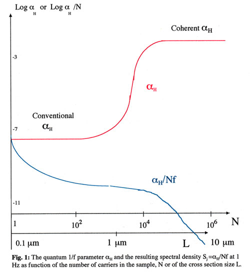
larger image
The question arises then: How far does one need to physically distance two longitudinal halves of the current-carrying sample, mentally separated along the center plane parallel to the current flow, in order to preclude the influence of the carriers from either half on the aH of those in the other half?
This mutual enhancement of 1/f noise from 2 samples in the transition region between the predominantly coherent and the mainly conventional crosss section sizes is what we will call "Induced 1/f Noise", or "Quantum 1/f Proximity Effect". The effect is proportional to the mutual inductance M12 between the two parallel halves, or between two parallel currents at a distance d in general. This is shown in Sec. VI below. The interaction between carriers, that is introduced by the magnetic field, causes the coherence present in the coherent quantum 1/f effect. There is a similarity between coherent quantum 1/f noise power and magnetic energy, or between conventional quantum 1/f noise and the kinetic energy of the drift motion. The total magnetic energy is not a sum of the contributions of individual carriers, but rather proportional to the square of such a coherent sum, i.e., to the squared magnetic field.
In conclusion, we expect the induced 1/f noise effect to vary with the distance d between two parallel elements of current proportionally to the mutual induction coefficient. This is applicable, e.g., to bundles of doped strands of DNA, used as conductors.
II. Introduction to quantum 1/f noise
Fluctuations with a spectral density proportional to 1/f are found in a large number of systems in science, technology and everyday life. These fluctuations are known as 1/f noise in general. They have first been noticed by Johnson1 in early amplifiers, have limited the performance of vacuum tubes in the thirties and forties, and have later hampered the introduction of semiconductor devices. They are often found in nature2, but they are causing particularly severe limitations to nanostructures and nano-scale devices.
Today the nature of 1/f noise is becoming quite well understood3-15 by us. There are some non-fundamental spectra that resemble 1/f noise over certain limited frequency intervals, and there is the fundamental 1/f noise that is ubiquitous. The non-fundamental (accidental) 1/f-like spectra are occasionally obtained in a limited frequency interval as a fortuitous superposition of Lorentzian spectra of the form 1/(1+w2t2, arising from exponential decay processes with autocorrelation functions of the form e-t/t. The fundamental 1/f spectra have been shown3 by us in general to arise at low frequencies from the simultaneous presence, or coincidence, of nonlinearity and of a dimensional homogeneity of a special kind. This coincidence is expressed by our sufficient criterion, providing the epistemological basis of 1/f spectra. The criterion allows us to determine whether a system defined by an arbitrary set of nonlinear integro-differential equations will have a 1/f spectrum. This criterion can also be seen as a consequence of the idempotent property of 1/f spectra with respect to autoconvolutions.
A special case of this fundamental 1/f noise is quantum 1/f noise, that is caused by the electrodynamical quantum 1/f effect3-20 (Q1/fE). The latter is of great technical, scientific and practical importance and has two limiting forms which are described with simple formulas, in more detail, below: conventional (for small devices) and coherent (for large devices) quantum 1/f effect.
The Q1/fE characterizes the form in which electrical charges, and matter (gravidynamical Q1/fE) in general, exist in space and time. It arises from the interaction of electrical charges with their field. The Q1/f E is therefore as fundamental as the notion of scattering, or as the notion of interaction (or "existence," in general).
Although it is a special case of fundamental 1/f noise, being caused by the simultaneous presence of nonlinearity and homogeneity in quantum electrodynamics at low frequencies, as defined by the sufficient criterion, it is the most fundamental from the ontological point of view. That is the point of view that constructs the universe from quarks and leptons, or, based on string theory. In particular, the Q1/fE is more fundamental than thermal noise, and it even modulates5 the level of Nyquist (or Johnson) noise in current or voltage (but not in available power), to yield the physical thermal noise.
III Conventional Quantum 1/f Effect
This effect3-9, 13-15 is present in any cross section or process rate involving charged particles or current carriers. The physical origin of quantum 1/f noise is easy to understand. Consider for example Coulomb scattering of current carriers, e.g., electrons on a center of force. The scattered electrons reaching a detector at a given angle away from the direction of the incident beam are described by DeBroglie waves of a frequency corresponding to their energy. However, some of the electrons have lost energy in the scattering process, due to the emission of bremsstrahlung. Therefore, part of the outgoing DeBroglie waves is shifted to slightly lower frequencies. When we calculate the probability density in the scattered beam, we obtain also cross terms, linear both in the part scattered with and without bremsstrahlung. These cross terms oscillate with the same frequency as the frequency of the emitted bremsstrahlung photons. The emission of photons at all frequencies results therefore in probability density fluctuations at all frequencies. The corresponding current density fluctuations are obtained by multiplying the probability density fluctuations by the velocity of the scattered current carriers. Finally, these current fluctuations present in the scattered beam will be noticed at the detector as low frequency current fluctuations, and will be interpreted as fundamental cross section fluctuations in the scattering cross section of the scatterer. While incoming carriers may have been Poisson distributed, the scattered beam will exhibit super-Poissonian statistics, or bunching, due to this new effect which we may call quantum 1/f effect. The quantum 1/f effect is thus a many-body or collective effect, at least a two-particle effect, best described through the two-particle wave function and two-particle correlation function.
Let us estimate the magnitude of the quantum 1/f effect semiclassically by starting with the classical (Larmor) formula 2q2a2/3c3 for the power radiated by a particle of charge q and acceleration a. The acceleration can be approximated by a delta function a(t) = Dvd(t) whose Fourier transform Dv is constant and is the change in the velocity vector of the particle during the almost instantaneous scattering process. The one-sided spectral density of the emitted bremsstrahlung power 4q2(Dv)2/3c3 is therefore also constant. The number 4q2(Dv)2/3hfc3 of emitted photons per unit frequency interval is obtained by dividing with the energy hf of one photon. The probability amplitude of photon emission [4q(Dv)2/ 3hfc3]1/2eig is given by the square root of this photon number spectrum, including also a phase factor eig. Let y be a representative Schrödinger catalogue wave function of the scattered outgoing charged particles, which is a single-particle function, normalized to the actual scattered particle concentration. The beat term in the probability density r=|y|2 is linear both in this bremsstrahlung amplitude and in the non-bremsstrahlung amplitude. Its spectral density will therefore be given by the product of the squared probability amplitude of photon emission (proportional to 1/f) with the squared non-bremsstrahlung amplitude which is independent of f. The resulting spectral density of fractional probability density fluctuations is obtained by dividing with |y|4 and is therefore
| |y|-4S|y|2(f) = 8q2(Dv)2/3hfNc3 = 2aA/fN = j-2Sj(f) |
(4) |
where a = e2/ c = 1/137 is the fine structure constant and aA = 4q2(Dv)2/3hc3 is known as the infrared exponent in quantum field theory, and is known as the quantum 1/f noise coefficient, in electrophysics. The experimentally measured quantity depends on many superposition or averaging processes and is often called, for historical reasons, Hooge constant. c = 1/137 is the fine structure constant and aA = 4q2(Dv)2/3hc3 is known as the infrared exponent in quantum field theory, and is known as the quantum 1/f noise coefficient, in electrophysics. The experimentally measured quantity depends on many superposition or averaging processes and is often called, for historical reasons, Hooge constant.
The spectral density of current density fluctuations is obtained by multiplying the probability density fluctuation spectrum with the squared velocity of the outgoing particles. When we calculate the spectral density of fractional fluctuations in the scattered current j, the outgoing velocity simplifies, and therefore Eq. (4) also gives the spectrum of current fluctuations Sj(f), as indicated above. The quantum 1/f noise contribution of each carrier is independent. Therefore the quantum 1/f noise from N carriers is N times larger. However, the current j will also be N times larger. Therefore in Eq. (4) a factor N was included in the denominator for the case in which the cross section fluctuation is observed with the help of N carriers that define the scattered current.
The fundamental fluctuations of cross sections and process rates are reflected in various kinetic coefficients in condensed matter, such as the mobility m and the diffusion constant D, the surface and bulk recombination speeds s, and recombination times t, the rate of tunneling jt and the thermal diffusivity in semiconductors. Therefore, the spectral density of fractional fluctuations in all these coefficients is given also by Eq. (4).
When we apply Eq. (4) to a certain device, we first need to find out which are the cross sections s or process rates that limit the current I through the device, or which determine any other device parameter P of interest. Second, we have to determine both the velocity change Dv of the scattered carriers and the number N of carriers used to test each of these cross sections or rates. Then Eq. (4) provides the spectral density of quantum 1/f cross section (or rate) fluctuations. These spectral densities are multiplied by the squared partial derivatives ( I/s)2 of the current, or (P/s)2 of any device parameter P of interest, to obtain the spectral density of fractional device noise contributions from the cross sections and rates considered. After doing this with all cross sections and process rates, we add the results and bring (factor out) the fine structure constant a as a common factor in front. This yields excellent agreement with the experiment9 in a large variety of samples, devices and physical systems. I/s)2 of the current, or (P/s)2 of any device parameter P of interest, to obtain the spectral density of fractional device noise contributions from the cross sections and rates considered. After doing this with all cross sections and process rates, we add the results and bring (factor out) the fine structure constant a as a common factor in front. This yields excellent agreement with the experiment9 in a large variety of samples, devices and physical systems.
Eq. (4) was also derived in second quantization7,8, using the commutation rules for boson field operators. For fermions one repeats the calculation replacing in the derivation the commutators of field operators by anticommutators, which yields7,8
| r-2Sr(f) = j-2Sj(f) = s-2Ss(f) = 2aA/f(N-1) |
(5) |
This causes no difficulties, since N 2 for particle correlations to be defined, and is practically the same as Eq. (4), since usually N>>1. Eqs. (4) and (5) introduce new quantum mechanical notions of "physical cross sections and process rates" which contain 1/f noise, and express a fundamental law of physics, important in most high-technology applications8, 13-15. 2 for particle correlations to be defined, and is practically the same as Eq. (4), since usually N>>1. Eqs. (4) and (5) introduce new quantum mechanical notions of "physical cross sections and process rates" which contain 1/f noise, and express a fundamental law of physics, important in most high-technology applications8, 13-15.
We conclude that the conventional quantum 1/f effect can be explained in terms of interference beats. The interference is between the part of the outgoing DeBroglie waves scattered without bremsstrahlung energy losses above the detection limit (given in turn by the reciprocal duration T of the 1/f noise measurement) on one hand, and the various parts scattered with bremsstrahlung energy losses. However, there is more to it than that: exchange between identical particles is also important.
This, of course, is just one way to describe the reaction of the emitted bremsstrahlung back on the scattered current. This reaction, itself an expression of the nonlinearity introduced by the coupling of the charged-particle field to the electromagnetic field, reveals itself here as the cause of the quantum 1/f effect, and implies that the effect can not be obtained with an "independent boson model". The effect, just like the classical turbulence-generated 1/f noise12, is a result of the scale-invariant nonlinearity of the equations of motion describing the coupled system of matter and field. Ultimately, therefore, this nonlinearity is the source of the 1/f spectrum in both the classical (turbulence) and quantum form of the theory. We can say that the quantum 1/f effect is an infrared divergence phenomenon, this divergence being the result of the same nonlinearity. The quantum 1/f effect is, in fact, the first time-dependent infrared radiative correction. Finally, it is also deterministic in the sense of a well-determined wave function, once the initial phases g of all field oscillators are given. In quantum mechanical correspondence with its classical turbulence analog12, the new effect is therefore a quantum manifestation of classical chaos which we can take as the definition of a certain type of quantum chaos, that is very fundamental.
IV Elementary application to homogeneous semiconductor samples.
In a homogeneous sample of length L, cross section A, volume V=AL, carrier mobility m, carrier concentration n and total number of carriers N=nAL, the conductance C=nmeA/L and the resistance R=1/C will exhibit quantum 1/f fluctuations. Their spectral density SdC/C of fractional fluctuations dC/C = -dR/R is given by
| SdC/C(f) = SdR/R(f) = Sdm/m(f) = ao/fN |
(6) |
To calculate ao we first evaluate the parameter s = nA·5.5·10-13 cm introduced in Sec. V below. If s1, coherent quantum 1/f noise (see Sec. V below) is observed with ao= 2a/p. If s<<1, Eq. (6) requires knowledge of (ao)conv. The latter is calculated from Eq. (4) or (5) for each type of scattering which limits the mobility m = et/m* of the carriers. Here t is the mean collision time or scattering time of the carriers and m* is their effective mass. In terms of the mean frequency of collisions n = 1/t = svni, one obtains m = e/nm* = e/svnim*. Here v is the mean speed of the carriers between collisions, s a scattering cross section and ni the concentration of scatterers.
Conventional Q1/fE in the mobility. In general, Matthiessen' rule allows us to write, in terms of mobility,
1/m =  1/mj 1/mj |
(7) |
where mj is the mobility which would be obtained if only the j-th scattering mechanism would be present and would limit the mobility. Applying a quantum 1/f fluctuation to Eq. (7), squaring and averaging quantum mechanically and statistically, we obtain as a reasonable first approximation
| dm/m2 = dmj/mj2 |
; |
Sdm/m(f) = (m/mj)2Sdm/mj(f). |
(8) |
Eq. (5) yields the strongest conventional quantum 1/f noise for umklapp scattering, followed by the f and g forms of inter-valley scattering or inter-valley with umklapp (in indirect band gap semiconductors like Si and Ge only). This is followed in this order by normal phonon scattering, by neutral impurity scattering and by ionized impurity scattering (that has lowest 1/f noise). The corresponding terms in Eq. (8) reflect this hierarchy only partially, because of the factors (m/mj)2 which gauge the importance of each of the scattering processes in limiting the resultant mobility. The conventional quantum 1/f effect present in the various scattering processes is estimated below.
Impurity scattering. For instance, in the case of impurity scattering, ni is the concentration of impurity atoms and ions. One obtains Sdm/m(f) = Sds/s(f). The physical scattering cross section s, in turn, exhibits the Q1/fE with the spectral density given by Eqs. (4) and (5)
Sds/s(f)i = (4a/3pfN)<[Dv/c]2> (3·10-3/fN)( Dk/m*c)2 (3·10-3/fN)( Dk/m*c)2 |
(9) |
The average quadratic velocity change of the electrons in a scattering process is smaller in impurity scattering than in lattice scattering which includes normal phonon scattering, inter-valley scattering in indirect band gap semiconductors with several "valleys", and umklapp scattering, as well as optical phonon scattering. The Coulomb/Rutherford or Conwell/Weiskopf type scattering cross section is proportional to 1/|Dk|4, which favors small angle scattering. Nevertheless, there are a few larger angle scattering events which are most effective in limiting the mobility and which therefore are decisive in the exact evaluation of the Q1/fE coefficient as a slow function of ni, the concentration of impurities, given in the theory section below. This corresponds approximately to assuming randomizing collisions,
| <(Dv)2>i = 2<v2> =6kBT/m* |
(10) |
although impurity scattering is not randomizing. With mo representing the free electron mass, we obtain this way
| Sdm/m(f)i = Sds/s(f)i = (4a/3pfN)<[6kBT/m*c2]>(10-9/fN)(Tmo/4m*100K). |
(11) |
The quantum 1/f noise power present in impurity scattering is therefore proportional to T.
Normal acoustic phonon scattering. For normal phonon scattering, the product svni has to be replaced by the lattice scattering rate G, given by an effective number of phonons times the squared phonon scattering matrix element, |M|2. The latter exhibits quantum 1/f fluctuations, because the carriers emit bremsstrahlung photons in the scattering process. Therefore, if the mobility m of electrons (of random velocity v = k/m*) is limited by phonon scattering, we get
| Sdm/m(f)ap = SdG/G(f)ap = (4a/3pfN)<(Dk/m*c)2> = (3·10-3/fN)<(Dq/m*c)2>. |
(12) |
Here Dq is the acoustic phonon momentum transfer in the scattering process and the brackets indicate the average value. Using the linear approximation of the acoustic phonon dispersion relation Eq=vsq, with vs denoting the speed of sound, we obtain for a thermal phonon with Eq=kBT/2
| <(Dq/m*c)2>.= (kBT/2vsm*c)2 = 1.25·10-5 (mo/m*)2 |
(13) |
We finally obtain
| Sdm/m(f)ap = (3.75·10-8/fN)(mo/m*)2 |
(14) |
The mean square momentum change and the 1/f noise are much larger (e.g., 50 times) for acoustic phonon scattering, because impurity scattering is mainly small-angle scattering.
Umklapp scattering. In this case the momentum change is close to the smallest reciprocal lattice vector approximated by G=2p/a, where a is the lattice constant. Therefore, Eq. (9) yields
| (aoU)conv = (4a/3p)[2p/am*c]2 = (6·10-8/fN)(mo/m*)2. |
(15) |
for Umklapp scattering.
Inter-valley scattering. In indirect band gap semiconductors the location of the energy minima of the conduction band in k-space is different from the location of the valence band energy maxima. In thermal equilibrium electrons and holes are present close to the minima of the conduction and valence bands. Scattering processes carrying electrons from one minimum (or valley) to the other are known as inter-valley scattering. This is large-angle scattering, compared with normal (intra-valley) scattering, and it is therefore affected by larger conventional quantum 1/f noise, almost as large as Umklapp scattering. Indeed, e.g., in Si the 8 minima are located at 0.85G from the origin, where G is the smallest reciprocal lattice vector. For g-processes which scatter an electron to the valley symmetrically located on the other side of the origin, Eq. (15) remains valid with a correction factor of (0.85)2. On the other hand for f-processes in Si, scattering electrons between to neighboring valleys, the factor is 2 times smaller. There is also the possibility of inter-valley scattering with umklapp which requires a correction factor of (1-0.85)2. Eq. (15) thus yields for inter-valley scattering with Umklapp
| (aoIU)conv = 0.0225 (4a/3p)[2p/am*c]2 = (1.35·10-9/fN)(mo/m*)2 |
(16) |
While this appears to indicate a lower contribution from these inter-valley umklapp processes, the corresponding (m/mj)2 factor in Eq. (18) insures a larger contribution to the resulting spectral density of quantum 1/f noise Sdm/m(f). Physically, this is caused by the scarcity of high-energy phonons able to bridge the momentum gap of 0.85G.
V. Physical Derivation of the Coherent Quantum 1/f Effect, and its Relation to the Conventional Q1/fE
This effect arises in a beam of electrons (or other charged particles propagating freely in vacuum) from the definition of the physical electron as a bare particle plus a coherent state of the electromagnetic field10. It is caused by the energy spread characterizing any coherent state of the electromagnetic field oscillators, an energy spread which spells non-stationarity, i.e., fluctuations. To find the spectral density of these inescapable fluctuations that are known to characterize any quantum state which is not an energy eigenstate, we use an elementary physical derivation based on Schrödinger's definition of coherent states. This supplements a rigorous derivation3,13-15 which was given from a well-known quantum-electrodynamical propagator.
The coherent quantum 1/f effect will be derived10 in three steps: first we consider a hypothetical world with just one single mode of the electromagnetic field, coupled to a beam of charged particles. Considering the mode to be in a coherent state, we calculate the autocorrelation function of the quantum fluctuations in the particle-density (or concentration, and current) that arise from the nonstationarity of the coherent state. Then we calculate the amplitude with which this one mode is represented in the field of an electron, according to electrodynamics. Finally, we take the product of the autocorrelation functions calculated for all modes with the amplitudes found in the previous step.
Let a mode of the electromagnetic field be characterized by the wave vector q, the angular frequency w = cq and the polarization l. Denoting the variables q and l simply by q in the labels of the states, we write the coherent state of amplitude |zq| and phase arg zq in the form
| |zq> = exp[-(1/2)|zq|2] exp[zqaq+] |0> = exp[-(1/2)|zq|2] /n! |n>. |
(17) |
Here aq+ is the creation operator which adds one energy quantum to the energy of the mode. Let us use a representation of the energy eigenstates in terms of Hermite polynomials Hn(x)
|n> = (2nn!  p)-1/2 exp[-x2/2] Hn(x) einwt. p)-1/2 exp[-x2/2] Hn(x) einwt. |
(18) |
This yields for the coherent state |zq> the representation
| yq(x) =exp[-(1/2)|zq|2]exp[-x2/2]Hn(x)=exp[-|zq|2/2]exp[-x2/2]exp[-zq2e-2iwt +2xzqeiwt]. |
(19) |
In the last form the generating function of the Hermite polynomials was used. The corresponding autocorrelation function of the probability density function, obtained by averaging over the time t or the phase of zq, is, for |zq|<<1,
| Pq(t,x) = <|yq|t2 | yq|t+t2 > = {1 + 8x2|zq|2[1 + cos wt] - 2|zq|2}exp[-x2/2]. |
(20) |
Integrating over x from - to , we find the autocorrelation function to , we find the autocorrelation function
| A1(t) = (2)-1/2{1 + 2|zq|2cos wt}. |
(21) |
This result shows that the probability distribution contains a constant background with small superposed oscillations of frequency w. Physically, the small oscillations in the total probability describe self-organization or bunching of the particles in the beam. They are thus more likely to be found in a measurement at a certain time and place than at other times and places relative to each other along the beam. Note that in the absence of the charge (e=0), for zq = 0 the coherent state becomes the ground state of the oscillator which is also an energy eigenstate, and therefore stationary and free of oscillations.
We now determine the amplitude zq with which the field mode q is represented in the physical electron. One way to do this is to let a bare particle dress itself through its interaction with the electromagnetic field, i.e. by performing first order perturbation theory with the interaction Hamiltonian
| H' = Am jm = -(e/c)v·A + ef, |
(22) |
where A is the vector potential and f the scalar electric potential. Another way is to Fourier expand the electric potential e/r of a charged particle in a box of volume V. In both ways we obtain the well-known result
| |zq|2 = p(e/q)2(cqV)-1. |
(23) |
Considering now all modes of the electromagnetic field, we obtain from the single - mode result of Eq. (21)
A(t) =CPq{1 +2|zq|2cos wqt} =C{1 +Sq 2|zq|2cos wqt} =C{1 + 4(V/23p3) d3q|zq|2cos wqt}. d3q|zq|2cos wqt}. |
(24) |
Here we have again used the smallness of zq and we have introduced a constant C. Using Eq. (23) we obtain
| A(t) = C{1 +4p(V/23p3)(4p/V)(e2/c) (dq/q)cos wqt} =C{1 + 2(a/p cos(wt)dw/w}. |
(25) |
Here a = e2/c is Sommerfeld's fine structure constant 1/137. The first term in curly brackets is unity and represents the constant background, or the d.c. part of the current carried by the beam of particles through vacuum. The autocorrelation function for the relative (fractional) density fluctuations, or for the current density fluctuations in the beam of charged particles is obtained therefore by dividing the second term in curly brackets by the first term. The constant C drops out when the fractional fluctuations are considered. According to the Wiener-Khintchine theorem, the coefficient of coswt is the spectral density of the fluctuations, S|y|2 for the particle concentration, or Sj for the current density j = e(k/m)|y|2
| S|y|2<|y|-2> =Sj<j>-2 =2(a/pfN) =4.6·10-3 f-1N-1. |
(26) |
Here we have included the total number N of charged particles which are observed simultaneously in the denominator, because the noise contributions from each particle are independent. This result is related to the conventional Quantum 1/f Effect considered in the next section. A similar calculation yields the gravidynamical quantum 1/f effect (QGD 1/f effect) by substituting gravitons for the photons considered so far as infraquanta.
Relation to the coherent Quantum 1/f Effect. We turn now to the connection11 with the coherent Quantum 1/f Effect. The coherent state in a conductor or semiconductor sample is the result of the experimental efforts directed towards establishing a steady and constant current, and is therefore the state defined by the collective motion, i.e. by the drift of the current carriers. It is expressed in the Hamiltonian by the magnetic energy Em, per unit length, of the current carried by the sample. In very small samples or electronic devices, this magnetic energy
| Em = (B2/8p)d3x = [nevS/c]2ln(R/r) |
(27) |
is much smaller than the total kinetic energy Ek of the drift motion of the individual carriers
| Ek = Smv2/2 = nSmv2/2 = Em/s. |
(28) |
Here we have introduced the magnetic field B, the carrier concentration n, the cross sectional area S and radius r of the cylindrical sample (e.g., a current carrying wire), the radius R of the electric circuit, and the "coherece ratio"
s  Em/Ek = 2ne2S/mc2ln (R/r) 2e2N'/mc2, Em/Ek = 2ne2S/mc2ln (R/r) 2e2N'/mc2, |
(29) |
where N' = nS is the number of carriers per unit length of the sample and the natural logarithm ln(R/r) has been approximated by one in the last form. We expect the observed spectral density of the mobility fluctuations to be given by a relation of the form
| (1/m2)Sm(f) = [1/(1+s)][2aA/fN] + [s/(1+s)][2a/pfN] |
(30) |
that can be interpreted as an expression of the effective Hooge constant if the number N of carriers in the (homogeneous) sample is brought to the numerator of the left hand side. In this equationaA=2a(Dv/c)2/3p is the usual nonrelativistic expression of the infrared exponent, present in the familiar form of the conventional quantum 1/f effect3-8. This equation is limited to quantum 1/f mobility (or diffusion) fluctuations, and does not include the quantum 1/f effect in the surface and bulk recombination cross sections, in the surface and bulk trapping centers, in tunneling and injection processes, in emission or in transitions between two solids. The latter also includes the quantum 1/f contact noise. All these effects are often misunderstood and misinterpreted as "number of carriers fluctuations" and misused as arguments against the "mobility fluctuations model of 1/f noise. In fact, they are all manifestations of the fundamental quantum 1/f noise, with the above-mentioned exception of accidental 1/f-like spectra.
Note that the coherence ratio s introduced here equals the unity for the critical value N' =N" = 2·1012/cm., e.g. for a cross section S = 2·10-4 cm2 of the sample when n = 1016. For small samples with N'<<N" only the first term survives, while for N'>N" the second term in Eq. (38.40) is dominant.
VI. Proximity Effect
Consider now two very long straight conductors of length L, of almost equal circular cross sections S1 and S2S1, both with approximate radius of the cross section r, carrying currents I1 =nevS1 and I2 =nevS2 and separated by a distance a between their axes. Then the magnetic energy in Eq. (27) becomes, per unit length,
| Em =(1/L)(B2/8p)d3x [(nevS1/c)+(nevS2/c)]2ln(R/r) -2(nevS1/c)(nevS2/c)ln(a/r). |
(31) |
Substituting a/r=(R/r)(a/R) in Eq. (31), we obtain
| Em [(nevS1/c)2+(nevS2/c)2]ln(R/r) +2(nevS1/c)(nevS2/c)ln(R/a). |
(32) |
Here R is a practically infinite large cutoff of the order of the radius of the circuit that contains the straight conductor of length L. Notice that for a=r, when the two conductors are in contact, the second term in Eq. (31) is zero and the magnetic energy is the well-known energy of a single cylindrical conductor of circular cross section S of radius r. On the other hand, for a=R the second term can be combined with the first term in Eq. (31) to yield simply the sum of the energies of the two infinitely separated parallel conductors. The approximation indicated in Eq. (31) uses the same effective radius r in the argument of the slowly varying logarithm present in the first term, as is used for each of the conductors separately. Note, however, that using 2r or r2 would ignore the additional magnetic energy caused by currents present inside the 2r or r2 radius, close to r, where the 2 conductors touch each other. That would severely under-estimate the magnetic energy.
The second term in Eq. (31) is the interaction energy of the two conductors, given by minus the work Wm done by us in the separation process against the electrodynamical attraction force between the conductors,
| Wm = Fda = (2I1I2/ac2)da, |
(32) |
when the distance is increased from r to a. The integral from r to a in Eq. (32) yields the second term in Eq. (31) with opposite sign. The negative sign appears because in the separation process, the induced-Faraday-emf work Wb done by the system of energy W=SIiFi/2 on the agency (e.g. a battery) to keep the currents constant is twice as large than Wm, and of opposite sign. In fact, while we are doing the separation work Wm on the system of two conductors, the system, in turn, must do on the battery twice the work Wm performed by us on itself, for the benefit of the agency that keeps the current constant in the two conductors. Indeed, denoting the fluxes through the circuits to which the two parallel conductors are belonging with F1 and f2 respectively,
| dW(I=const) =SIidFi/2; |
dWb(I=const) = S IidFi; |
dWm(I=const) =-SIidFi/2 |
(33) |
with the sum S runs over i=1 and 2, we obtain for the differential dW of the energy W of the system of two conductors in the form
This explains the minus sign in Eq. (31).
Based on symmetry and S2S1, we use Eq. (32) to write the magnetic energy corresponding to the first conductor
| Em1 (nevS1/c)2ln(R/r) +(nevS1/c)(nevS2/c)ln(R/a). |
(35) |
The last term can be written in terms of the mutual inductance as I1I2M12. To generalize the definition of the parameter s of Eq. (29) we divide Eq. (35) by the kinetic energy of the drift component present in the motion of current carriers in the first conductor, per unit length
| Ek1 = Smv2/2 = nS1mv2/2. |
(36) |
This yields
| sEm1/Ek1 2ne2S1/mc2ln(R/r)+2(ne2S2/mc2)ln(R/a), |
(37) |
or
| s s1 + s2{[ln(R/a)]/[ln(R/r)]}. |
(38) |
This form clearly displays the proximity effect in the second term of the expression obtained for the s-parameter in the presence of a similar current located at the distance a. From the observation following Eq. (35), we can see that the proximity effect is proportional to the mutual inductance M12 between the two parallel conductors.
REFERENCES
1. J.B. Johnson, "The Schottky-Effect in Low-Frequency Circuits", Phys. Rev. 26, 71-85 (1925).
2. W.H. Press, Comments Astrophys, Space Phys. 7, 103 (1978).
3. P.H. Handel: "The Nature of Fundamental 1/f Noise", XII. Internatl. Conf. on Noise in Physical Systems and 1/f Fluctuations, St. Louis, MO, Aug. 16-20, 1993, AIP Conf. Proceedings No. 285, P.H. Handel and A.L. Chung, Editors, pp. 162-171 (1993).
4. P.H. Handel: "1/f Noise - an 'Infrared' Phenomenon", Phys. Rev. Letters 34, 1492 - 1494 (1975); "Nature of 1/f Phase Noise", Phys. Rev. Letters 34, 1495-1498 (1975).
5. P.H. Handel: "Quantum Approach to 1/f Noise", Phys. Rev. 22A, p. 745 (1980).
6. P.H. Handel and D. Wolf: "Characteristic Functional of Quantum 1/f Noise", Phys. Rev. A26, 3727-30 (1982).
7. P.H. Handel: "The Quantum 1/f Effect and the General Nature of 1/f Noise", Archiv für Elektronik und Übertragungstechnik (AEÜ) 43, 261-270 (1989);
8. T.S. Sherif and P.H. Handel: "Unified Treatment of Diffraction and 1/f Noise", Phys. Rev. A26, p.596-602, (1982).
9. A. van der Ziel, "Unified Presentation of 1/f Noise in Electronic Devices; Fundamental 1/f Noise Sources", Proc. IEEE 76, 233-258 (1988 review paper); "The Experimental Verification of Handel's Expressions for the Hooge Parameter", Solid-State Electronics 31, 1205-1209 (1988); "Semiclassical Derivation of Handel's Expression for the Hooge Parameter", J. Appl. Phys. 63, 2456-2455 (1988); 64, 903-906 (1988); A.N. Birbas et al., J. Appl. Phys. 64, 907-912 (1988); A. van der Ziel et. al., "Extensions of Handel's 1/f Noise Equations and their Semiclassical Theory", Phys. Rev. B 40, 1806-1809 (1989); M. Tacano, Proc. XI. Int. Conf. on Noise in Physical Systems and 1/f Fluctuations, T. Musha, S. Sato and Y. Mitsuaki Editors, Ohmsha Publ. Co., Tokyo 1991, pp. 167-170; M. Tacano, Proc. Fifth van der Ziel Conference "Quantum 1/f Noise and other Low Frequency Fluctuations" AIP Conference proceedings #282, P.H. Handel and A.L. Chung Editors, 1992; see also "Quantum 1/f Bibliography" by P.H. Handel, unpublished.
10. P.H. Handel, "Any Particle Represented by a Coherent State Exhibits 1/f Noise" in "Noise in Physical Systems and 1/f Noise", (Proceedings of the VIIth International Conference on Noise in Physical Systems and 1/f Noise) edited by M. Savelli, G. Lecoy and J.P. Nougier (North - Holland, Amsterdam, 1983), p. 97.
11. P.H. Handel, "Coherent States Quantum 1/f Noise and the Quantum 1/f Effect" in "Noise in Physical Systems and 1/f Noise" (Proceedings of the VIIIth International Conference on Noise in Physical Systems and 1/f Noise) edited by A. D'Amico and P. Mazzetti, Elsevier, New York, 1986, p. 469.
12. P.H. Handel: "Instabilities, Turbulence and Flicker-Noise in Semiconductors I, II and III", Zeitschrift für Naturforschung 21a, 561-593 (1966); P.H. Handel: "Turbulence Theory for the Current Carriers in Solids and a Theory of 1/f Noise", Phys. Rev. A3, 2066 (1971).
13. P.H. Handel: "Noise, Low Frequency", Wiley Encyclopedia of Electrical and Electronics Engineering, vol. 14, pp. 428-449, John Wiley & Sons, Inc., John G. Webster, Editor, 1999.
14. P.H. Handel: "Coherent and Conventional Quantum 1/f Effect" Physica Status Solidi b194, pp. 393-409 (1996)
15. P.H. Handel: "Fundamental Quantum 1/f Noise in Semiconductor Devices", IEEE Trans. on Electr. Devices 41, 2023-2033 (1994).
16. C.M. Van Vliet: "Quantum Electrodynamical Theory of Infrared Effects in Condensed Matter. I & II" Physica A 165, 101-125, 126-155(1990).
17. A. Van der Ziel, "Unified Presentation of 1/f Noise in Electronic Devices; Fundamental 1/f Noise Sources", Proc. IEEE 76, 233-258 (1988); (review paper) and "Noise in Solid State Devices and Circuits", J. Wiley & Sons, New York 1986, Ch. 11, pp. 254 - 277.
18. A. van der Ziel, "The Experimental Verification of Handel's Expressions for the Hooge Parameter", Solid State Electronics, 31,1205-1209 (1988).
19. A. van der Ziel, A.D. van Rheenen, and A.N. Birbas, "Extensions of Handel's 1/f Noise Equations and their Semiclassical Theory", Phys. Rev. B40, 1806-1809 (1989).
20. P.H. Handel: "Noise, Low Frequency", Wiley Encyclopedia of Electrical and Electronics Engineering, vol. 14, pp. 428-449, John Wiley & Sons, Inc., John G. Webster, Editor, 1999.
|